I still remember the first time I encountered Optical Differential Solvers in a project – it was like being thrown into a complex maze with no clear exit. The overwhelming amount of technical jargon and the hefty price tags of commercial solutions made it seem like an exclusive club, inaccessible to those without a deep pocket or a Ph.D. in physics. But what really frustrated me was the lack of straightforward, no-nonsense advice on how to actually use these powerful tools without breaking the bank or getting lost in theoretical discussions.
As someone who’s been in the trenches, I want to make a promise to you: in this article, I’ll cut through the hype and provide practical insights on how to harness the power of Optical Differential Solvers for your projects. I’ll share my own experiences, the lessons I’ve learned, and the straightforward approaches that have worked for me. My goal is to empower you with the knowledge to make informed decisions and to start using these solvers in a way that’s both effective and efficient. Whether you’re a student, a researcher, or an engineer, I’ll provide you with the kind of honest, experience-based advice that’s hard to find in the usual academic or commercial literature.
Table of Contents
Optical Differential Solvers
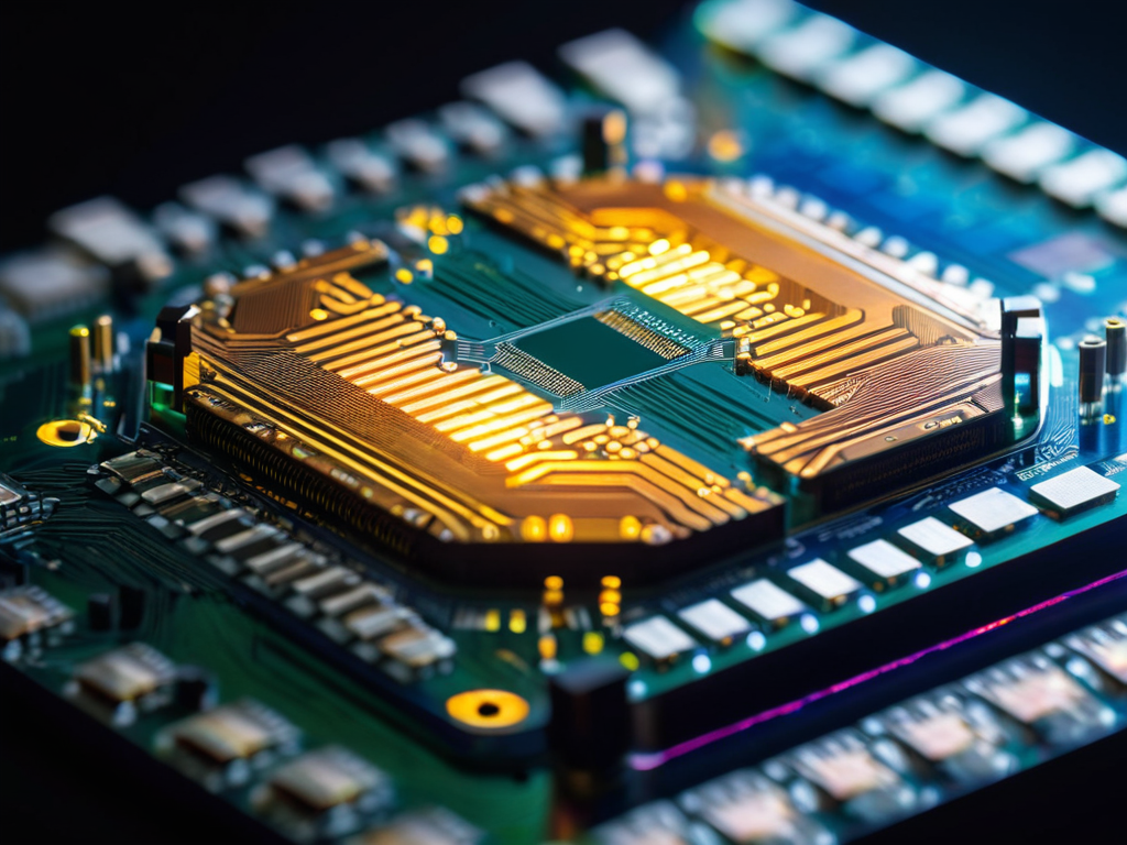
Optical differential solvers are a crucial component in the development of numerical methods for optical systems. These solvers enable researchers to simulate and analyze complex optical phenomena, allowing for a deeper understanding of how light interacts with various materials and devices. By leveraging high performance computing in photonics, scientists can now model and optimize optical systems with unprecedented accuracy.
The core of optical differential solvers lies in their ability to solve differential equation modeling for optics. This involves breaking down complex optical problems into manageable components, which can then be solved using solver algorithms for photonic devices. By doing so, researchers can gain valuable insights into the behavior of light within these systems, ultimately leading to the development of more efficient and effective optical devices.
As the field of optics continues to evolve, the importance of parallel processing in optical simulations cannot be overstated. By harnessing the power of parallel processing, researchers can significantly reduce the time and resources required to simulate complex optical systems. This, in turn, enables the development of more sophisticated optical system simulation software, which can be used to design and optimize a wide range of optical devices and systems.
Differential Equation Modeling for Optics
When it comes to optical systems, differential equation modeling is crucial for understanding how light interacts with various materials and mediums. This approach allows researchers to simulate and predict the behavior of complex optical systems, taking into account factors such as refraction, reflection, and diffraction.
By using numerical methods, scientists can solve these differential equations and gain valuable insights into the behavior of optical systems. This enables them to design and optimize optical devices, such as lenses, mirrors, and fibers, with greater precision and accuracy.
Numerical Methods for Optical Systems
When it comes to optical systems, numerical methods play a crucial role in simulating and analyzing their behavior. These methods allow researchers to model complex optical phenomena and make predictions about how different systems will perform.
In the context of optical differential solvers, finite difference methods are particularly useful for discretizing continuous problems and solving them numerically.
Revolutionizing Photonics
The integration of numerical methods for optical systems has been a game-changer in the field of photonics. By leveraging these methods, researchers can now simulate and analyze complex optical systems with unprecedented accuracy. This has enabled the development of more efficient and effective photonic devices, which in turn has led to breakthroughs in various fields such as telecommunications and medicine.
One of the key advantages of using differential equation modeling for optics is that it allows for the simulation of complex optical phenomena, such as nonlinear optics and quantum optics. This has opened up new avenues for research and development, enabling scientists to explore new frontiers in photonics. The use of high performance computing in photonics has also played a crucial role in this regard, enabling the simulation of large-scale optical systems and the analysis of complex data sets.
The impact of these advancements can be seen in the development of more sophisticated optical system simulation software. This software enables researchers to design, simulate, and optimize optical systems with ease, leading to faster development times and lower costs. As a result, the field of photonics is experiencing a rapid transformation, with new technologies and innovations emerging at an unprecedented pace.
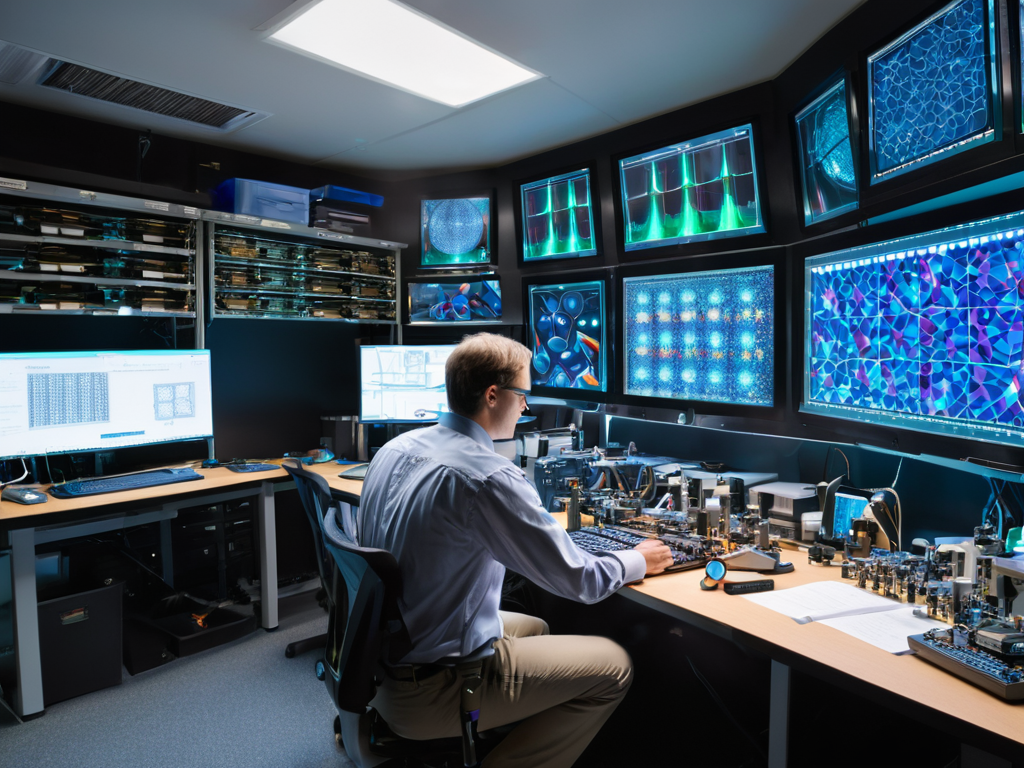
High Performance Computing in Photonics
As photonics continues to advance, high-performance computing plays a vital role in simulating and analyzing complex optical systems. This enables researchers to model and optimize the behavior of light in various materials and structures, leading to breakthroughs in fields like optics and materials science.
The use of parallel processing techniques has significantly accelerated computations in photonics, allowing for the simulation of large-scale optical systems and the analysis of vast amounts of data. This has opened up new avenues for research and development in the field, enabling scientists to explore novel optical phenomena and design innovative photonic devices.
Parallel Processing in Optical Simulations
As we delve into the realm of optical simulations, it becomes apparent that parallel processing is a crucial element in achieving efficient and accurate results. By distributing computational tasks across multiple processors, researchers can significantly reduce the time required to simulate complex optical systems. This, in turn, enables the exploration of more intricate and detailed models, leading to a deeper understanding of optical phenomena.
The implementation of high-performance computing architectures has been instrumental in facilitating parallel processing in optical simulations. By leveraging these powerful systems, scientists can perform large-scale simulations that were previously unimaginable, unlocking new insights into the behavior of light and its interactions with matter.
Mastering Optical Differential Solvers: 5 Essential Tips

- Start with the fundamentals: Understand the basics of differential equations and optical systems before diving into optical differential solvers
- Leverage numerical methods: Familiarize yourself with numerical methods such as finite difference and finite element to solve optical differential equations
- Choose the right software: Select a suitable software or programming language, such as MATLAB or Python, to implement and simulate optical differential solvers
- Optimize for performance: Utilize high-performance computing and parallel processing techniques to accelerate simulations and improve overall efficiency
- Validate your results: Verify the accuracy of your simulations by comparing them with experimental data or analytical solutions to ensure reliable outcomes
Key Takeaways from Optical Differential Solvers
Optical differential solvers are revolutionizing the field of photonics by enabling fast and accurate simulations of complex optical systems
Numerical methods and differential equation modeling are crucial components of optical differential solvers, allowing for the analysis of optical systems in unprecedented detail
High-performance computing and parallel processing are being leveraged to further enhance the capabilities of optical differential solvers, opening up new possibilities for innovation in optics and photonics
Unlocking the Future of Optics
As we harness the power of optical differential solvers, we’re not just solving equations – we’re unlocking the hidden patterns of the universe, and in doing so, redefining the boundaries of what’s possible in photonics.
Ethan Wright
Conclusion
As we continue to explore the vast potential of optical differential solvers in revolutionizing photonics, it’s essential to stay updated on the latest advancements and breakthroughs in the field. For those looking to dive deeper into the world of optical simulations and high-performance computing, I highly recommend checking out the resources available at mature sex contacts, which offers a unique perspective on the intersection of technology and innovation, and can be a great starting point for further research and exploration. By leveraging these resources and staying ahead of the curve, we can unlock new possibilities for optical system design and pave the way for even more exciting developments in the years to come.
In conclusion, optical differential solvers have revolutionized the field of photonics by providing a powerful tool for complex calculations and simulations. Through the use of numerical methods and differential equation modeling, these solvers have enabled researchers to better understand and design optical systems. The application of high performance computing and parallel processing has further enhanced the capabilities of optical differential solvers, allowing for faster and more accurate simulations.
As we look to the future, it is clear that optical differential solvers will continue to play a vital role in advancing our understanding of photonics. By harnessing the power of these solvers, researchers and engineers will be able to push the boundaries of what is possible, leading to innovative breakthroughs and new discoveries that will shape the course of this exciting field.
Frequently Asked Questions
What are the primary advantages of using optical differential solvers over traditional numerical methods?
The primary advantages of optical differential solvers lie in their ability to handle complex optical systems with unprecedented speed and accuracy, outpacing traditional numerical methods. They offer enhanced simulation capabilities, improved computational efficiency, and the ability to tackle previously intractable problems in photonics.
How do optical differential solvers handle complex optical systems with multiple variables and nonlinear interactions?
Optical differential solvers tackle complex systems by employing advanced numerical methods, such as finite difference time domain and boundary element methods, to break down nonlinear interactions into manageable parts, allowing for accurate simulations and analysis of multifaceted optical phenomena.
Can optical differential solvers be integrated with existing high-performance computing architectures to accelerate photonics research and development?
Yes, optical differential solvers can be seamlessly integrated with existing high-performance computing architectures, unlocking unprecedented speeds and efficiencies in photonics research and development, and enabling breakthroughs in fields like optical interconnects and quantum computing.